Data analysis

These are XPPAUT's Numerics > stocHastic and Numerics > Averaging tools, run by XPPAUT's own code. Each one analyses the model's last run, as XPPAUT's menus do, and leaves the run unchanged. Most return a Table: named NumPy columns, with .to_pandas() and .plot().

import xpplab as xs
m = xs.load("lecar.ode")
m.run(total=400)

Spectra

m.fourier("V")                  # freq, cos, sin: the Fourier series of V
m.power("V")                    # freq, amplitude, phase
m.spectrum("V", length=512)     # Welch power spectral density
m.spectrum("V", "W", kind="coherence", length=256, window="hann")

fourier and power treat the whole run as one period: frequencies are mode k divided by the length of the run. spectrum averages the FFTs of windows of length points that overlap by half (XPPAUT's Spec.dns). kind is "psd", "cross" (the size of the cross spectrum) or "coherence"; window is "square", "parzen", "hamming" (the default), "bartlett" or "hann".

Histograms, correlations, statistics

m.histogram("V", bins=50)                    # bin (left edge), count
m.histogram("V", bins=50, condition="W>0.2") # count only where W > 0.2
m.histogram2d("V", "W", bins=(20, 20))       # x, y, fraction of points
m.correlation("V", lags=100)                 # autocorrelation: lag, correlation
m.correlation("V", "W", lags=100, fft=True)  # cross-correlation by FFT
mean, sd = m.mean("V")

Ranges default to the column's range in the run; pass range=(lo, hi) to fix them. The correlations subtract the means (they are covariances) and give lags in time units.

Liapunov exponent

m = xs.load("lorenz.ode")
m.run(total=200)
m.lyapunov()                    # about 0.9: chaos

XPPAUT's estimate of the largest exponent: a small perturbation is carried along the run one output step at a time and renormalised, and the logs of its growth are averaged. Use a long run that has settled onto the attractor; the result is negative for a stable equilibrium and near zero on a limit cycle.

Phase response curves

m.apply_set("snic")
m.parameters["iapp"] = 0.09
prc = m.phase_response()
prc.plot("V")                   # against phase, 0 to 1
prc.period                      # 23.87

phase_response does what XPPAUT users do by hand:

1. Integrate past the transient onto the limit cycle (transient= defaults to the model's total time).
2. Measure the period from the upward crossings of the first variable (or variable=), or take period=.
3. Integrate exactly one period. This is m.limit_cycle(), which leaves that period as the run.
4. Compute XPPAUT's adjoint along it: m.adjoint().

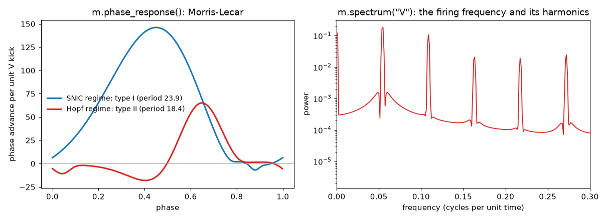
Each variable's column is the infinitesimal phase response curve to perturbations of that variable: how much a small kick advances the next event, per unit of kick, in time units. XPPAUT normalises the adjoint so that its dot product with the vector field is 1. Divide by prc.period for the phase response in cycles.

In the figure, Morris-Lecar near a saddle-node on an invariant circle (SNIC) has a type I PRC: kicks only advance it. Near a Hopf bifurcation it has a type II PRC: early kicks delay it.

Weakly coupled oscillators: the H function

prc = m.phase_response()
h = m.h_function({"V": "V'-V", "W": "0"})   # gap-junction coupling through V
h.plot()

After the adjoint, h_function averages the coupling over one cycle to give the interaction function H(phi) of the phase model dθ/dt = ω + ε H(θ̂ − θ). Give one formula per variable; primed names (V') are the other oscillator's variables. For three or more columns the table also has the odd and even parts, Hodd and Heven. For two identical, symmetrically coupled oscillators the phase difference obeys dφ/dt = −2ε Hodd(φ), so the zeros of Hodd where it slopes upward are the stable phase-locked states.

Fitting a model to data

fitted = m.fit("recording.dat", variables="V", parameters=["gca", "gk"])

Levenberg-Marquardt, as in XPPAUT's stocHastic > fIt data. The data are a file or an array with time in the first column. variables are the model variables to match and columns their columns in the data (by default 2, 3, ...). parameters lists the parameters, and initial conditions, to vary. They start from their current values, end at the fitted ones, and are returned as a dict. The model's initial conditions apply at the first data time, and XPPAUT integrates from each data time to the next with the current method, so the data need not be evenly spaced.

Range: many runs over a parameter

runs = m.sweep("iapp", np.linspace(0, 0.2, 21))              # 21 Trajectories
peaks = m.sweep("iapp", np.linspace(0, 0.2, 21),
                measure=lambda s: s["V"].max())              # an array
lyap = m.sweep("r", np.linspace(20, 30, 31), measure=lambda s: m.lyapunov(),
               continue_runs=True)                           # chaos onset

sweep is XPPAUT's Initial conds > Range. The name can be a parameter or a variable (its initial value). With continue_runs=True each run starts where the last ended ("Use old ICs" = No), so a branch is followed as the parameter moves. Each run equals XPPAUT's batch range digit for digit. m.ic_last() alone is XPPAUT's Initial conds > Last.

Boundary-value problems

m = xs.load("cable.ode")    # v'' = v, with bndry v-1 and bndry v'
sol = m.bvp()               # shooting from the initial values as a guess
m.get("VX")                 # the initial slope that solves it

For models with bndry statements, bvp() runs XPPAUT's shooting method over [T0, T0 + total]. On success the initial conditions hold the solution's and the solution is returned.

Animations and 3D

m = xs.load("pend.ode")
m.run(total=20)
ani = m.animation("pend.ani")   # parsed and evaluated by XPPAUT
ani.frame(100)                  # the shapes at row 100: lines, ellipses, ...
ani.plot(100)                   # one frame with matplotlib
ani.save_gif("pend.gif")        # an animated GIF (needs Pillow)

xs.load("lorenz.ode").run().plot3d("X", "Y", "Z")

Each shape has its coordinates in the animation's window (ani.window, 0..1 unless the file says dimension) and a matplotlib colour.