Phase plane

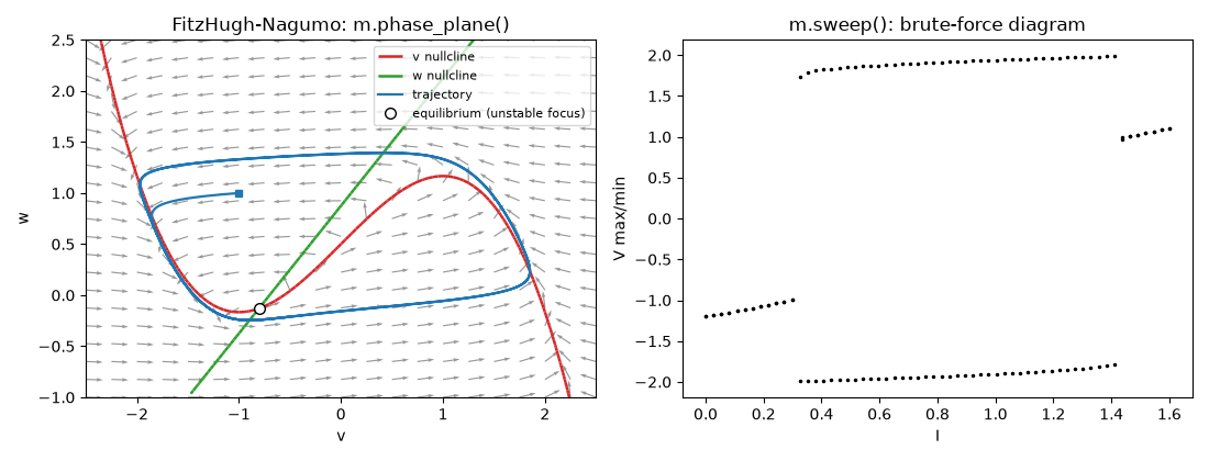
One call

ax = m.phase_plane("v", "w", xlim=(-2.5, 2.5), ylim=(-1, 2.5))

draws the trajectory, both nullclines, the direction field and the nearest equilibrium (filled if stable, open if not). Each part can be switched off: nullclines=False, field=False, trajectory=False, equilibrium=False. Pass ax= to draw into your own axes.

The pieces

xn, yn = m.nullclines("v", "w", (-2.5, 2.5), (-1, 2.5), grid=150)

returns two arrays of line segments, each of shape (n, 4) holding x1, y1, x2, y2. They come from XPPAUT's own contouring algorithm. Draw them with matplotlib's LineCollection(xn.reshape(-1, 2, 2)).

X, Y, U, V = m.vector_field("v", "w", (-2.5, 2.5), (-1, 2.5), n=20)
plt.quiver(X, Y, U, V)

f = m.rhs({"v": 0.5, "w": 0.2})     # dv/dt and dw/dt at a point

In models with more than two variables, the variables not on the axes keep their initial values.

Nullclines as a parameter changes

values = np.linspace(0, 0.4, 6)
frozen = m.nullcline_sweep("iapp", values, "V", "W", (-0.6, 1.2), (-0.25, 1.2))
m.phase_plane("V", "W", xlim=(-0.6, 1.2), ylim=(-0.25, 1.2), frozen=frozen)
xs.Table.from_nullclines(frozen, first=1).to_csv("nc.csv")

nullcline_sweep is XPPAUT's Nullcline > Freeze > Range: one (x_nullcline, y_nullcline) pair per value, the parameter put back afterwards. phase_plane(frozen=...) draws such pairs faded behind the live nullclines. Table.from_nullclines lists the segments, one row each (set, nullcline 1 or 2, x1, y1, x2, y2), as the desktop app's export nc.csv nullclines writes them.

Equilibria

eq = m.equilibrium()                     # start from the initial values
eq = m.equilibrium({"v": 1.0, "w": 0.5}) # or from a guess
eq.values           # {'V': ..., 'W': ...}
eq.eigenvalues      # complex NumPy array
eq.stable, eq.kind  # False, 'unstable focus'
m.equilibrium(set_initial=True)          # also make it the initial value

kind is one of: stable node, unstable node, stable focus, unstable focus, saddle, saddle-focus. For maps it is stable or unstable.

Every equilibrium, and equilibria over a parameter

eqs = m.find_equilibria(guesses=200, box={"V": (-0.6, 0.6), "W": (-0.1, 0.8)})
eqs                 # <3 equilibria: unstable focus, saddle, stable node>
eqs.to_csv("eqs.csv")

t = m.equilibrium_sweep("iapp", np.linspace(0, 0.3, 31))
t.columns           # ['iapp', 'V', 'W', 'unstable', 'stable']

find_equilibria is XPPAUT's Sing pts > Monte Carlo: Newton's method from random points in a box (variables left out of box span -10 to 10, XPPAUT's default), keeping each distinct equilibrium. XPPAUT's random numbers repeat, so the same call finds the same list.

equilibrium_sweep is Sing pts > Range: at each value the search starts from the equilibrium found at the value before. The table gives the numbers of unstable and stable eigenvalues; where no equilibrium was found the row holds NaN. The parameter is restored afterwards.